Chapter 11 : Transportation

Chapter 11 : Transportation

Multiple Fact Table Granularity

When it comes to the grain, we encounter a situation in this case where we are

presented with multiple potential levels of fact table granularity. Each of these

levels of granularity has different metrics associated with them.

At the most granular level, the airline captures data at the leg level. The leg

represents an aircraft taking off at one airport and landing at another without

any intermediate stops. Capacity planning and flight scheduling analysts are

very interested in this discrete level of information because they’re able to look

at the number of seats to calculate load factors by leg. We also can include facts

regarding the leg’s flight duration as well as the number of minutes late at

departure and arrival. Perhaps there’s even a dimension to easily identify

on-time arrivals.

The next level of granularity corresponds to a segment. In this case we’re

looking at the portion of a trip on a single aircraft. Segments may have one or

more legs associated with them. If you take a flight from San Francisco to

Minneapolis with a stop in Denver but no aircraft change, you have flown one

segment (SFO-MSP) but two legs (SFO-DEN and DEN-MSP). Conversely, if

the flight flew nonstop from San Francisco to Minneapolis, you would have

flown one segment as well as one leg. The segment represents the line item on

an airline ticket coupon; revenue and mileage credit is generated at the segment

level.

Next, we can analyze flight activity by trip. The trip provides an accurate picture

of customer demand. In our prior example, assume that the flights from

San Francisco to Minneapolis required the flyer to change aircraft in Denver. In

this case the trip from San Francisco to Minneapolis would entail two segments

corresponding to the two aircraft involved. In reality, the passenger just

asked to go from San Francisco to Minneapolis; the fact that he or she needed

to stop in Denver was merely a necessary evil but certainly wasn’t requested.

For this reason, sales and marketing analysts are interested in trip-level data.

Linking Segments into Trips

Despite the powerful dimensional framework we just designed, we are unable

to easily answer one of the most important questions about our frequent flyers,

namely, where are they going? The segment grain masks the true nature of

the trip. If we fetch all the segments of the airline voyage and sequence them

by segment number, it is still nearly impossible to discern the trip start and end

points. Most complete itineraries start and end at the same airport. If a lengthy

stop were used as a criterion for a meaningful trip destination, it would

require extensive and tricky processing whenever we tried to summarize a

number of voyages by the meaningful stops.

The answer is to introduce two more airport role-playing dimensions: trip origin

and trip destination, while keeping the grain at the flight segment level.

These are determined during data extraction by looking on the ticket for any

stop of more than four hours, which is the airline’s official definition of a

stopover. The enhanced schema looks like Figure 11.2. We would need to exercise

some caution when summarizing data by trip in this schema. Some of the

dimensions, such as fare basis or class of service flown, don’t apply at the trip

level. On the other hand, it may be useful to see how many trips from San

Francisco to Minneapolis included an unrestricted fare on a segment

In addition to linking segments into trips as Figure 11.2 illustrates, if the business

users are constantly looking at information at the trip level, rather than by segment,

we might be tempted to create an aggregate fact table at the trip grain.

Some of the earlier dimensions discussed, such as class of service, fare basis, and

flight, obviously would not be applicable. The facts would include such metrics

as trip gross revenue and additional facts that would appear only in this complementary

trip summary table, such as the number of segments in the trip.

However, we would only go to the trouble of creating such an aggregate table if

there were obvious performance or usability issues when we used the segmentlevel

table as the basis for rolling up the same reports. If a typical trip consisted

of three segments, then we might barely see a three times performance improvement

with such an aggregate table, meaning that it may not be worth the bother.

Cargo Shipper

The schema for a cargo shipper looks quite similar to the frequent flyer schemas

just developed. Suppose that a transoceanic shipping company transports bulk

goods in containers from foreign to domestic ports. The items in the containers

are shipped from an original shipper to a final consignor. The trip can have multiple

stops at intermediate ports. It is possible that the containers may be offloaded

from one ship to another at a port. Likewise, it is possible that one or

more of the legs may be by truck rather than ship.

As illustrated in Figure 11.3, the grain of the fact table is the container on a specific

bill-of-lading number on a particular leg of its trip.

The ship mode dimension identifies the type of shipping company and specific

vessel. The item dimension contains a description of the items in a container.

The container dimension describes the size of the container and whether it

requires electrical power or refrigeration. The commodity dimension describes

one type of item in the container. Almost anything that can be shipped can be

described by harmonized commodity codes, which are a kind of master conformed

dimension used by agencies, including U.S. Customs. The consignor

foreign transporter, foreign consolidator, shipper, domestic consolidator,

domestic transporter, and consignee are all roles played by a master business

entity dimension that contains all the possible business parties associated with

a voyage. The bill-of-lading number is a degenerate dimension. We assume that

the fees and tariffs are applicable to the individual leg of the voyage.

Travel Services

If we work for a travel services company, we can envision complementing the

customer flight activity schema with fact tables to track associated hotel stays

and rental car usage. These schemas would share several common dimensions,

such as the date, customer, and itinerary number, along with ticket and

segment number, as applicable, to allow hotel stays and car rentals to be interleaved

correctly into a airline trip. For hotel stays, the grain of the fact table is

the entire stay, as illustrated in Figure 11.4. The grain of a similar car rental fact

table would be the entire rental episode. Of course, if we were constructing a

fact table for a hotel chain rather than a travel services company, the schema

would be much more robust because we’d know far more about the hotel property

characteristics, the guest’s use of services, and associated detailed charges

Combining Small Dimensions into a Superdimension

We stated previously that if a many-to-many relationship exists between two

groups of dimension attributes, then they should be modeled as separate

dimensions with separate foreign keys in the fact table. Sometimes, however,

we’ll encounter a situation where these dimensions can be combined into a

single superdimension rather than treating them as two separate dimensions

with two separate foreign keys in the fact table

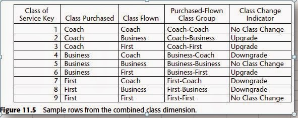
Class of Service

The Figure 11.1 draft schema included the class of service flown dimension. Following

our first design checkpoint with the business community, we learn that

the business users want to analyze the class of service purchased, as well as the

class flown. Unfortunately, we’re unable to reliably determine the class of service

actually used from the original fare basis because the customer may do a

last-minute upgrade. In addition, the business users want to easily filter and

report on activity based on whether an upgrade or downgrade occurred. Our

initial reaction is to include a second role-playing dimension and foreign key in

the fact table to support access to both the purchased and flown class of service,

along with a third foreign key for the upgrade indicator. In this situation, however,

there are only three rows in each class dimension table to indicate first,

business, and coach classes. Likewise, the upgrade indicator dimension also

would have just three rows in it, corresponding to upgrade, downgrade, or no

class change. Since the row counts are so small, we elect instead to combine the

dimensions into a single class of service dimension, as illustrated in Figure 11.5.

In most cases, role-playing dimensions should be treated as separate logical dimensions

created via views on a single physical table, as we’ve seen earlier with date

dimensions. In isolated situations it may make sense to combine the separate

dimensions into a superdimension, notably when the data volumes are extremely

small or there is a need for additional attributes that depend on the combined

underlying roles for context and meaning.

Country-specific calendar outrigger.

If there’s no need to roll up or filter on time-of-day groups, then we have the

option to treat time as a simple numeric fact instead. In this situation, the time

of day would be expressed as a number of minutes or number of seconds since

midnight, as shown in Figure 11.8

Date and Time in Multiple Time Zones

When operating in multiple countries or even just multiple time zones, we’re

faced with a quandary concerning transaction dates and times. Do we capture

the date and time relative to local midnight in each time zone, or do we express

the time period relative to a standard, such as the corporate headquarters

date/time or Greenwich Mean Time (GMT)? To fully satisfy users’ requirements,

the correct answer is probably both. The standard time allows us to see

the simultaneous nature of transactions across the business, whereas the local

time allows us to understand transaction timing relative to the time of day.

Contrary to popular belief, there are more than 24 time zones (corresponding

to the 24 hours of the day) in the world. For example, there is a single time

zone in India, offset from GMT by 5.5 or 6.5 hours depending on the time of

year. The situation gets even more unpleasant when you consider the complexities

of switching to and from daylight saving time. As such, it’s unreasonable

to think that merely providing an offset in a fact table can support

equivalized dates and times. Likewise, the offset can’t reside in a time or airport

dimension table. The recommended approach for expressing dates and

times in multiple time zones is to include separate date and time-of-day

dimensions (or time-of-day facts, as we just discussed) corresponding to the

local and equivalized dates, as shown in Figure 11.9.