DW Concepts -- Kimball & Ross - The Data Warehouse Toolkit

This post is kind abridged version [in our way] of first 15 chapters  of Book - Kimball & Ross - The Data Warehouse Toolkit. We have tried to pull out main points from each chapters, however somewhere if you will out of context or doesn't get a link, we request you to go through a respective chapter once.

Chapter 1 : Dimensional Modeling Primer

Basic Elements of Data Warehouse

ODS
In either scenario, the ODS can be either a third physical system sitting between
the operational systems and the data warehouse or a specially administered hot
partition of the data warehouse itself. Every organization obviously needs
Dimensional Modeling Primer 15
operational systems. Likewise, every organization would benefit from a data
warehouse. The same cannot be said about a physically distinct ODS unless the
other two systems cannot answer your immediate operational questions.
Clearly, you shouldn’t allocate resources to construct a third physical system
unless your business needs cannot be supported by either the operational datacollection
system or the data warehouse. For these reasons, we believe that the
trend in data warehouse design is to deliver the ODS as a specially administered

portion of the conventional data warehouse.

Cube
If the presentation area is based on a relational database, then these dimensionally
modeled tables are referred to as star schemas. If the presentation area
is based on multidimensional database or online analytic processing (OLAP)
technology, then the data is stored in cubes. While the technology originally
wasn’t referred to as OLAP, many of the early decision support system vendors
built their systems around the cube concept, so today’s OLAP vendors
naturally are aligned with the dimensional approach to data warehousing.
Dimensional modeling is applicable to both relational and multidimensional
databases. Both have a common logical design with recognizable dimensions;
however, the physical implementation differs. Fortunately, most of the recommendations
in this book pertain, regardless of the database platform. While
the capabilities of OLAP technology are improving continuously, at the time of
this writing, most large data marts are still implemented on relational databases.
In addition, most OLAP cubes are sourced from or drill into relational
dimensional star schemas using a variation of aggregate navigation

Facts

Additivity is crucial because data warehouse applications almost never

retrieve a single fact table row. Rather, they bring back hundreds, thousands,

or even millions of fact rows at a time, and the most useful thing to do with so

many rows is to add them up. In Figure 1.2, no matter what slice of the database

the user chooses, we can add up the quantities and dollars to a valid total.

We will see later in this book that there are facts that are semiadditive and still

others that are nonadditive. Semiadditive facts can be added only along some

of the dimensions, and nonadditive facts simply can’t be added at all. With

nonadditive facts we are forced to use counts or averages if we wish to summarize

the rows or are reduced to printing out the fact rows one at a time. This

would be a dull exercise in a fact table with a billion rows.

A row in a fact table corresponds to a measurement. A measurement is a row in a

fact table. All the measurements in a fact table must be at the same grain.

As we develop the examples in this book, we will see that all fact table grains

fall into one of three categories: transaction, periodic snapshot, and accumulating

snapshot. Transaction grain fact tables are among the most common

Snoflex Schema

Dimension tables often represent hierarchical relationships in the business. In

our sample product dimension table, products roll up into brands and then

into categories. For each row in the product dimension, we store the brand and

category description associated with each product. We realize that the hierarchical

descriptive information is stored redundantly, but we do so in the spirit

of ease of use and query performance. We resist our natural urge to store only

the brand code in the product dimension and create a separate brand lookup

table. This would be called a snowflake. Dimension tables typically are highly

denormalized.

Start Schema

Now that we understand fact and dimension tables, let’s bring the two building

blocks together in a dimensional model. As illustrated in Figure 1.4, the

fact table consisting of numeric measurements is joined to a set of dimension

tables filled with descriptive attributes. This characteristic starlike structure is

often called a star join schema. This term dates back to the earliest days of relational

databases.

Chapter 2 :  Retail

Four-Step Dimensional Design Process

1. Select the business process to model.

2. Declare the grain of the business process.

3. Choose the dimensions that apply to each fact table row

4. Identify the numeric facts that will populate each fact table row

Step 2. Declare the Grain

Once the business process has been identified, the data warehouse team faces

a serious decision about the granularity. What level of data detail should be

made available in the dimensional model? This brings us to an important

design tip.

Preferably you should develop dimensional models for the most atomic information

captured by a business process. Atomic data is the most detailed information collected;

such data cannot be subdivided further.

Why date dimentions are needed

Some designers pause at this point to ask why an explicit date dimension table

is needed. They reason that if the date key in the fact table is a date-type field,

then any SQL query can directly constrain on the fact table date key and use

natural SQL date semantics to filter on month or year while avoiding a supposedly

expensive join. This reasoning falls apart for several reasons. First of

all, if our relational database can’t handle an efficient join to the date dimension

table, we’re already in deep trouble. Most database optimizers are quite

efficient at resolving dimensional queries; it is not necessary to avoid joins like

the plague. Also, on the performance front, most databases don’t index SQL

date calculations, so queries constraining on an SQL-calculated field wouldn’t

take advantage of an index.

In terms of usability, the typical business user is not versed in SQL date semantics,

so he or she would be unable to directly leverage inherent capabilities

associated with a date data type. SQL date functions do not support filtering

by attributes such as weekdays versus weekends, holidays, fiscal periods, seasons,

or major events. Presuming that the business needs to slice data by these

nonstandard date attributes, then an explicit date dimension table is essential.

At the bottom line, calendar logic belongs in a dimension table, not in the

application code. Finally, we’re going to suggest that the date key is an integer

rather than a date data type anyway. An SQL-based date key typically is 8 bytes,

so you’re wasting 4 bytes in the fact table for every date key in every row. More

will be said on this later in this chapter.

Casual Dimension

Promotion Dimension

The promotion dimension is potentially the most interesting dimension in our

schema. The promotion dimension describes the promotion conditions under

which a product was sold. Promotion conditions include temporary price

reductions, end-aisle displays, newspaper ads, and coupons. This dimension

is often called a causal dimension (as opposed to a casual dimension) because

it describes factors thought to cause a change in product sales.

Null Values 

Typically, many sales transaction line items involve products that are not being

promoted. We will need to include a row in the promotion dimension, with its

own unique key, to identify “No Promotion in Effect” and avoid a null promotion

key in the fact table. Referential integrity is violated if we put a null in a

fact table column declared as a foreign key to a dimension table. In addition to

the referential integrity alarms, null keys are the source of great confusion to

our users because they can’t join on null keys.

You must avoid null keys in the fact table. A proper design includes a row in the

corresponding dimension table to identify that the dimension is not applicable

to the measurement

NonAdditive Facts

Percentages and ratios, such as gross margin, are nonadditive. The numerator and

denominator should be stored in the fact table. The ratio can be calculated in a data

access tool for any slice of the fact table by remembering to calculate the ratio of

the sums, not the sum of the ratios

Unit price is also a nonadditive fact. Attempting to sum up unit price across any

of the dimensions results in a meaningless, nonsensical number

Product Dimension

An important function of the product master is to hold the many descriptive

attributes of each SKU. The merchandise hierarchy is an important group of

attributes. Typically, individual SKUs roll up to brands. Brands roll up to

categories, and categories roll up to departments. Each of these is a many-toone

relationship. This merchandise hierarchy and additional attributes are

detailed for a subset of products in Figure 2.6.

Drill Down

A reasonable product dimension table would have 50 or more descriptive

attributes. Each attribute is a rich source for constraining and constructing row

headers. Viewed in this manner, we see that drilling down is nothing more

than asking for a row header that provides more information. Let’s say we

have a simple report where we’ve summarized the sales dollar amount and

quantity by department.

If we want to drill down, we can drag virtually any other attribute, such as

brand, from the product dimension into the report next to department, and we

automatically drill down to this next level of detail. Atypical drill down within

the merchandise hierarchy would look like this:

We have belabored the examples of drilling down in order to make a point,

which we will express as a design principle.

Drilling down in a data mart is nothing more than adding row headers from the

dimension tables. Drilling up is removing row headers. We can drill down or up on

attributes from more than one explicit hierarchy and with attributes that are part of

no hierarchy.

Degenerate dimension 

Although the POS transaction number looks like a dimension key in the fact

table, we have stripped off all the descriptive items that might otherwise fall in

a POS transaction dimension. Since the resulting dimension is empty, we refer

to the POS transaction number as a degenerate dimension (identified by the DD

notation in Figure 2.10). The natural operational ticket number, such as the

POS transaction number, sits by itself in the fact table without joining to a

dimension table. Degenerate dimensions are very common when the grain of

a fact table represents a single transaction or transaction line item because the

degenerate dimension represents the unique identifier of the parent. Order

numbers, invoice numbers, and bill-of-lading numbers almost always appear

as degenerate dimensions in a dimensional model.

Operational control numbers such as order numbers, invoice numbers, and bill-oflading

numbers usually give rise to empty dimensions and are represented as degenerate

dimensions (that is, dimension keys without corresponding dimension tables)

in fact tables where the grain of the table is the document itself or a line item in the

document.

Factless Fact table

Promotion Coverage Factless Fact Table

Regardless of the handling of the promotion dimension, there is one important

question that cannot be answered by our retail sales schema: What products

were on promotion but did not sell? The sales fact table only records the SKUs

actually sold. There are no fact table rows with zero facts for SKUs that didn’t

sell because doing so would enlarge the fact table enormously. In the relational

world, a second promotion coverage or event fact table is needed to help

answer the question concerning what didn’t happen. The promotion coverage

fact table keys would be date, product, store, and promotion in our case study.

This obviously looks similar to the sales fact table we just designed; however,

the grain would be significantly different. In the case of the promotion coverage

fact table, we’d load one row in the fact table for each product on promotion

in a store each day (or week, since many retail promotions are a week in

duration) regardless of whether the product sold or not. The coverage fact

table allows us to see the relationship between the keys as defined by a promotion,

independent of other events, such as actual product sales. We refer to

it as a factless fact table because it has no measurement metrics; it merely captures

the relationship between the involved keys. To determine what products

where on promotion but didn’t sell requires a two-step process. First, we’d

query the promotion coverage table to determine the universe of products that

were on promotion on a given day. We’d then determine what products sold

from the POS sales fact table. The answer to our original question is the set difference

between these two lists of products.

Snlowflaking

Dimension table normalization typically is referred to as snowflaking

The dimension tables should remain as flat tables physically. Normalized,

snowflaked dimension tables penalize cross-attribute browsing and prohibit the use

of bit-mapped indexes. Disk space savings gained by normalizing the dimension tables

typically are less than 1 percent of the total disk space needed for the overall

schema. We knowingly sacrifice this dimension table space in the spirit of performance

and ease-of-use advantages.

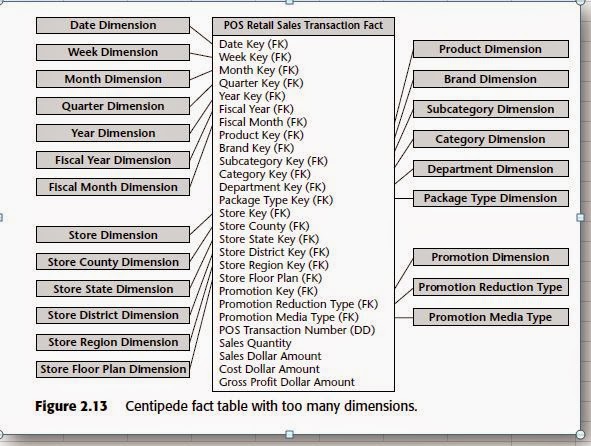
Centipede fact

Most business processes can be represented with less than 15 dimensions in

the fact table. If our design has 25 or more dimensions, we should look for

ways to combine correlated dimensions into a single dimension. Perfectly correlated

attributes, such as the levels of a hierarchy, as well as attributes with a

reasonable statistical correlation, should be part of the same dimension. You

have made a good decision to combine dimensions when the resulting new

single dimension is noticeably smaller than the Cartesian product of the separate

dimensions.

Chapter 3 : Inventory

Semiadditive Facts
We stressed the importance of fact additivity in Chapter 2. When we modeled
the flow of product past a point at the checkout cash register, only the products
that actually sold were measured. Once a product was sold, it couldn’t be
counted again in a subsequent sale. This made most of the measures in the
retail sales schema perfectly additive across all dimensions.
In the inventory snapshot schema, the quantity on hand can be summarized
across products or stores and result in a valid total. Inventory levels, however,
are not additive across dates because they represent snapshots of a level or balance
at one point in time. It is not possible to tell whether yesterday’s inventory
is the same or different from today’s inventory solely by looking at
inventory levels. Because inventory levels (and all forms of financial account
balances) are additive across some dimensions but not all, we refer to them as
semiadditive facts.
The semiadditive nature of inventory balance facts is even more understandable
if we think about our checking account balances. On Monday, let’s presume
that you have $50 in your account. On Tuesday, the balance remains
unchanged. On Wednesday, you deposit another $50 into your account so that
the balance is now $100. The account has no further activity through the end of
the week. On Friday, you can’t merely add up the daily balances during the
week and declare that your balance is $400 (based on $50 + 50 + 100 + 100 +
100). The most useful way to combine account balances and inventory levels
across dates is to average them (resulting in an $80 average balance in the
checking example). We are all familiar with our bank referring to the average
daily balance on our monthly account summary.
All measures that record a static level (inventory levels, financial account balances,
and measures of intensity such as room temperatures) are inherently nonadditive
across the date dimension and possibly other dimensions. In these cases, the measure
may be aggregated usefully across time, for example, by averaging over the
number of time periods.
Drill Across
In Chapters 1 and 2 we modeled data from several processes of the value
chain. While separate fact tables in separate data marts represent the data from
each process, the models share several common business dimensions, namely,
date, product, and store. We’ve logically represented this dimension sharing in
Figure 3.6. Using shared, common dimensions is absolutely critical to designing
data marts that can be integrated. They allow us to combine performance
measurements from different processes in a single report. We use multipass
SQL to query each data mart separately, and then we outer join the query
results based on a common dimension attribute. This linkage, often referred to
as drill across, is straightforward if the dimension table attributes are identical

Buss Architecture

The word bus is an old term from the electrical power industry that is now

used commonly in the computer industry. A bus is a common structure to

which everything connects and from which everything derives power. The bus

in your computer is a standard interface specification that allows you to plug

in a disk drive, CD-ROM, or any number of other specialized cards or devices.

Because of the computer’s bus standard, these peripheral devices work

together and usefully coexist, even though they were manufactured at different

times by different vendors.

By defining a standard bus interface for the data warehouse environment, separate

data marts can be implemented by different groups at different times. The separate

data marts can be plugged together and usefully coexist if they adhere to the standard

The bus architecture is independent of technology and the database platform.

All flavors of relational and online analytical processing (OLAP)-based data

marts can be full participants in the data warehouse bus if they are designed

around conformed dimensions and facts. Data warehouses will inevitably

consist of numerous separate machines with different operating systems and

database management systems (DBMSs). If designed coherently, they will

share a uniform architecture of conformed dimensions and facts that will

allow them to be fused into an integrated whole.

The major responsibility of the centralized dimension authority is to establish, maintain,

and publish the conformed dimensions to all the client data marts.

gross margin return on inventory (GMROI,pronounced “jem-roy”)

Although this formula looks complicated, the idea behind GMROI is simple. By

multiplying the gross margin by the number of turns, we create a measure of the

effectiveness of our inventory investment. A high GMROI means that we are

moving the product through the store quickly (lots of turns) and are making

good money on the sale of the product (high gross margin). Alow GMROI means

that we are moving the product slowly (low turns) and aren’t making very much

money on it (low gross margin). The GMROI is a standard metric used by inventory

analysts to judge a company’s quality of investment in its inventory.

If we want to be more ambitious than our initial design in Figure 3.2, then we

should include the quantity sold, value at cost, and value at the latest selling

price columns in our snapshot fact table, as illustrated in Figure 3.3. Of course,

if some of these metrics exist at different granularity in separate fact tables, a

requesting application would need to retrieve all the components of the

GMROI computation at the same level.

Notice that quantity on hand is semiadditive but that the other measures in

our advanced periodic snapshot are all fully additive across all three dimensions.

The quantity sold amount is summarized to the particular grain of the

fact table, which is daily in this case. The value columns are extended, additive

amounts. We do not store GMROI in the fact table because it is not additive.

We can calculate GMROI from the constituent columns across any number of

fact rows by adding the columns up before performing the calculation, but we

are dead in the water if we try to store GMROI explicitly because we can’t usefully

combine GMROIs across multiple rows.

Remember that there’s more to life than transactions alone. Some form of snapshot

table to give a more cumulative view of a process often accompanies a transaction

fact table.

Let’s assume that the inventory goes through a series of well-defined events or

milestones as it moves through the warehouse, such as receiving, inspection,

bin placement, authorization to sell, picking, boxing, and shipping. The philosophy

behind the accumulating snapshot fact table is to provide an updated

status of the product shipment as it moves through these milestones. Each fact

table row will be updated until the product leaves the warehouse. As illustrated

in Figure 3.5, the inventory accumulating snapshot fact table with its

multitude of dates and facts looks quite different from the transaction or periodic

snapshot schemas.

The rows of the bus matrix correspond to data marts. You should create separate

matrix rows if the sources are different, the processes are different, or if the matrix

row represents more than what can reasonably be tackled in a single implementation

iteration.

Creating the data warehouse bus matrix is one of the most important up-front deliverables

of a data warehouse implementation. It is a hybrid resource that is part technical

design tool, part project management tool, and part communication tool.

It goes without saying that it is unacceptable to build separate data marts that

ignore a framework to tie the data together. Isolated, independent data marts

are worse than simply a lost opportunity for analysis. They deliver access to

irreconcilable views of the organization and further enshrine the reports that

cannot be compared with one another. Independent data marts become legacy

implementations in their own right; by their very existence, they block the

development of a coherent warehouse environment.

Conformed Fact

Revenue, profit, standard prices, standard costs, measures of quality, measures

of customer satisfaction, and other key performance indicators (KPIs) are facts

that must be conformed. In general, fact table data is not duplicated explicitly

in multiple data marts. However, if facts do live in more than one location,

such as in first-level and consolidated marts, the underlying definitions and

equations for these facts must be the same if they are to be called the same

thing. If they are labeled identically, then they need to be defined in the same

dimensional context and with the same units of measure from data mart to

data mart.

Chapter 4 : Procruments

Type 1: Overwrite the Value

With the type 1 response, we merely overwrite the old attribute value in the

dimension row, replacing it with the current value. In so doing, the attribute

always reflects the most recent assignment.

The type 1 response is easy to implement, but it does not maintain any history of

prior attribute values.

Before we leave the topic of type 1 changes, there’s one more easily overlooked

catch that you should be aware of. When we used a type 1 response to deal

with the relocation of IntelliKidz, any preexisting aggregations based on the

department value will need to be rebuilt. The aggregated data must continue

to tie to the detailed atomic data, where it now appears that IntelliKidz has

always rolled up into the Strategy department.

Type 2: Add a Dimension Row

We made the claim earlier in this book that one of the primary goals of the data

warehouse was to represent prior history correctly. A type 2 response is the

predominant technique for supporting this requirement when it comes to

slowly changing dimensions.

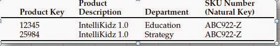
Using the type 2 approach, when IntelliKidz’s department changed, we issue

a new product dimension row for IntelliKidz to reflect the new department

attribute value. We then would have two product dimension rows for IntelliKidz,

such as the following:

Now we see why the product dimension key can’t be the SKU number natural

key. We need two different product surrogate keys for the same SKU or physical

barcode. Each of the separate surrogate keys identifies a unique product

attribute profile that was true for a span of time. With type 2 changes, the fact

table is again untouched. We don’t go back to the historical fact table rows to

modify the product key.

If we constrain only on the department attribute, then we very precisely differentiate

between the two product profiles. If we constrain only on the product

description, that is, IntelliKidz 1.0, then the query automatically will fetch

both IntelliKidz product dimension rows and automatically join to the fact

table for the complete product history. If we need to count the number of products

correctly, then we would just use the SKU natural key attribute as the

basis of the distinct count rather than the surrogate key. The natural key field

becomes a kind of reliable glue that holds the separate type 2 records for a single

product together. Alternatively, a most recent row indicator might be

another useful dimension attribute to allow users to quickly constrain their

query to only the current profiles.

Since the type 2 technique spawns new dimension rows, one downside of this

approach is accelerated dimension table growth. Hence it may be an inappropriate

technique for dimension tables that already exceed a million rows.

Type 3: Add a Dimension Column

In our software example, let’s assume that there is a legitimate business need

to track both the old and new values of the department attribute both forward

and backward for a period of time around the change. With a type 3 response,

we do not issue a new dimension row, but rather we add a new column to capture

the attribute change. In the case of IntelliKidz, we alter the product

dimension table to add a prior department attribute. We populate this new column

with the existing department value (Education). We then treat the department

attribute as a type 1 response, where we overwrite to reflect the current

value (Strategy). All existing reports and queries switch over to the new

department description immediately, but we can still report on the old department

value by querying on the prior department attribute.

The type 3 slowly changing dimension technique allows us to see new and historical

fact data by either the new or prior attribute values

Atype 3 response is inappropriate if you want to track the impact of numerous

intermediate attribute values.

Hybrid Slowly Changing Dimension Techniques

Each sales rep dimension row would include all prior district assignments.

The business user could choose to roll up the sales facts with any of the five

district maps. If a sales rep were hired in 2000, the dimension attributes for

1998 and 1999 would contain values along the lines of “Not Applicable.”

We label the most recent assignment as “Current District.” This attribute will

be used most frequently; we don’t want to modify our existing queries and

reports to accommodate next year’s change. When the districts are redrawn

next, we’d alter the table to add a district 2002 attribute. We’d populate this

column with the current district values and then overwrite the current

attribute with the 2003 district assignments.

In this manner we’re able to use the historical attribute to segment history and

see facts according to the departmental roll-up at that point in time. Meanwhile,

the current attribute rolls up all the historical fact data for product keys

12345 and 25984 into the current department assignment. If IntelliKidz were

then moved into the Critical Thinking software department, our product table

would look like the following:

With this hybrid approach, we issue a new row to capture the change (type

2) and add a new column to track the current assignment (type 3), where

subsequent changes are handled as a type 1 response. Someone once suggested

that we refer to this combo approach as type 6 (2 + 3 + 1). This technique

allows us to track the historical changes accurately while also

supporting the ability to roll up history based on the current assignments.

We could further embellish (and complicate) this strategy by supporting

additional static department roll-up structures, in addition to the current

department, as separate attributes.

More Rapidly Changing Dimensions

In this chapter we’ve focused on the typically rather slow, evolutionary

changes to our dimension tables. What happens, however, when the rate of

change speeds up? If a dimension attribute changes monthly, then we’re no

longer dealing with a slowly changing dimension that can be handled reasonably

with the techniques just discussed. One powerful approach for handling

more rapidly changing dimensions is to break off these rapidly changing

attributes into one or more separate dimensions. In our fact table we would

then have two foreign keys—one for the primary dimension table and another

for the rapidly changing attribute(s). These dimension tables would be associated

with one another every time we put a row in the fact table.

Chapter 5 : Order Management

Order management consists of several critical business processes, including

order, shipment, and invoice processing. These processes spawn important

business metrics, such as sales volume and invoice revenue, that are key performance

indicators for any organization that sells products or services to

others.

It is natural and common, especially for customer-oriented dimensions, for a dimension
to simultaneously support multiple independent hierarchies. The hierarchies
may have different numbers of levels. Drilling up and drilling down within each of
these hierarchies must be supported in a data warehouse.

The one-to-one or many-to-one relationship may turn out to be a many-tomany
relationship. As we discussed earlier, if the many-to-many relationship
is an exceptional condition, then we may still be tempted to combine
the sales rep attributes into the ship-to dimension, knowing that we’d need
to treat these rare many-to-many occurrences by issuing another surrogate
ship-to key.
If the relationship between sales rep and customer ship-to varies over time
or under the influence of a fourth dimension such as product, then the
combined dimension is in reality some kind of fact table itself! In this
case, we’d likely create separate dimensions for the sales rep and the customer
ship-to.
If the sales rep and customer ship-to dimensions participate independently
in other business process fact tables, we’d likely keep the dimensions
separate. Creating a single customer ship-to dimension with sales rep

attributes exclusively around orders data may make some of the other

Role Playing Dimension

Role-playing in a data warehouse occurs when a single dimension simultaneously

appears several times in the same fact table. The underlying dimension may exist as

a single physical table, but each of the roles should be presented to the data access

tools in a separately labeled view.

Deal Dimension
The deal dimension is similar to the promotion dimension from Chapter 2. The
deal dimension describes the incentives that have been offered to the customer
that theoretically affect the customers’ desire to purchase products. This
dimension is also sometimes referred to as the contract. As shown in Figure 5.4,
the deal dimension describes the full combination of terms, allowances, and

incentives that pertain to the particular order line item.

Degenerate Dimension for Order Number

Each line item row in the orders fact table includes the order number as a

degenerate dimension, as we introduced in Chapter 2. Unlike a transactional

parent-child database, the order number in our dimensional models is not tied

to an order header table. We have stripped all the interesting details from the

order header into separate dimensions such as the order date, customer ship-to,

and other interesting fields. The order number is still useful because it allows us

to group the separate line items on the order. It enables us to answer such questions

as the average number of line items on an order. In addition, the order

number is used occasionally to link the data warehouse back to the operational

world. Since the order number is left sitting by itself in the fact table without

joining to a dimension table, it is referred to as a degenerate dimension.

Degenerate dimensions typically are reserved for operational transaction identifiers.

They should not be used as an excuse to stick a cryptic code in the fact table without

joining to a descriptive decode in a dimension table.

Junk Dimensions

When we’re confronted with a complex operational data source, we typically

perform triage to quickly identify fields that are obviously related to dimensions,

such as date stamps or attributes. We then identify the numeric measurements

in the source data. At this point, we are often left with a number of

miscellaneous indicators and flags, each of which takes on a small range of discrete

values. The designer is faced with several rather unappealing options,

including:

Leave the flags and indicators unchanged in the fact table row. This could

cause the fact table row to swell alarmingly. It would be a shame to create a

nice tight dimensional design with five dimensions and five facts and then

leave a handful of uncompressed textual indicator columns in the row

Make each flag and indicator into its own separate dimension. Doing so

could cause our 5-dimension design to balloon into a 25-dimension design.

Strip out all the flags and indicators from the design. Of course, we ask the

obligatory question about removing these miscellaneous flags because they

seem rather insignificant, but this notion is often vetoed quickly because

someone might need them. It is worthwhile to examine this question carefully.

If the indicators are incomprehensible, noisy, inconsistently populated,

or only of operational significance, they should be left out

An appropriate approach for tackling these flags and indicators is to study

them carefully and then pack them into one or more junk dimensions.

A junk dimension is a convenient grouping of typically low-cardinality flags and indicators.

By creating an abstract dimension, we remove the flags from the fact table

while placing them into a useful dimensional framework.

We’ve illustrated sample rows from an order indicator dimension in Figure 5.5. A

subtle issue regarding junk dimensions is whether you create rows for all the

combinations beforehand or create junk dimension rows for the combinations as

you actually encounter them in the data. The answer depends on how many possible

combinations you expect and what the maximum number could be. Generally,

when the number of theoretical combinations is very high and you don’t

think you will encounter them all, you should build a junk dimension row at

extract time whenever you encounter a new combination of flags or indicators

Header and Line Item Facts with Different Granularity
It is quite common in parent-child transaction databases to encounter facts of differing
granularity. On an order, for example, there may be a shipping charge that
applies to the entire order that isn’t available at the individual product-level line
item in the operational system. The designer’s first response should be to try to
force all the facts down to the lowest level. We strive to flatten the parent-child
relationship so that all the rows are at the child level, including facts that are captured
operationally at the higher parent level, as illustrated in Figure 5.7. This procedure
is broadly referred to as allocating. Allocating the parent order facts to the
child line-item level is critical if we want the ability to slice and dice and roll up all
order facts by all dimensions, including product, which is a common requirement

We shouldn’t mix fact granularities (for example, order and order line facts) within a

single fact table. Instead, we need to either allocate the higher-level facts to a more

detailed level or create two separate fact tables to handle the differently grained

facts. Allocation is the preferred approach. Optimally, a finance or business team

(not the data warehouse team) spearheads the allocation effort.

Invoice Transaction

In the shipment invoice fact table we can see all the company’s products, all

the customers, all the contracts and deals, all the off-invoice discounts and

allowances, all the revenue generated by customers purchasing products, all

the variable and fixed costs associated with manufacturing and delivering

products (if available), all the money left over after delivery of product (contribution),

and customer satisfaction metrics such as on-time shipment.

For any company that ships products to customers or bills customers for services rendered,

the optimal place to start a data warehouse typically is with invoices. We often

refer to the data resulting from invoicing as the most powerful database because it

combines the company’s customers, products, and components of profitability.

Extended gross invoice amount. This is also know as extended list price

because it is the quantity shipped multiplied by the list unit price.

Extended allowance amount. This is the amount subtracted from the

invoice-line gross amount for deal-related allowances. The allowances are

described in the adjoined deal dimension. The allowance amount is often

called an off-invoice allowance

Extended discount amount. This is the amount subtracted on the invoice for

volume or payment-term discounts. The explanation of which discounts

are taken is also found in the deal dimension row that points to this fact

table row

All allowances and discounts in this fact table are represented at the line

item level. As we discussed earlier, some allowances and discounts may be

calculated operationally at the invoice level, not the line-item level. An

effort should be made to allocate them down to the line item. An invoice

P&L statement that does not include the product dimension poses a serious

limitation on our ability to present meaningful P&L slices of the business.

Extended net invoice amount. This is the amount the customer is expected to

pay for this line item before tax. It is equal to the gross invoice amount less

the allowances and discounts.

However, there are times when users are more interested in analyzing the

entire order fulfillment pipeline. They want to better understand product

velocity, or how quickly products move through the pipeline. The accumulating

snapshot fact table provides us with this perspective of the business, as

illustrated in Figure 5.10. It allows us to see an updated status and ultimately

the final disposition of each order

The accumulating snapshot complements our alternative perspectives of the

pipeline. If we’re interested in understanding the amount of product flowing

through the pipeline, such as the quantity ordered, produced, or shipped, we rely

on transaction schemas that monitor each of the pipeline’s major spigots. Periodic

snapshots give us insight into the amount of product sitting in the pipeline, such

as the backorder or finished goods inventories, or the amount of product flowing

through a spigot during a predefined time period. The accumulating snapshot

helps us better understand the current state of an order, as well as product movement

velocities to identify pipeline bottlenecks and inefficiencies.

We notice immediately that the accumulating snapshot looks different from

the other fact tables we’ve designed thus far. The reuse of conformed dimensions

is to be expected, but the number of date and fact columns is larger than

we’ve seen in the past. We capture a large number of dates and facts as the

order progresses through the pipeline. Each date represents a major milestone

of the fulfillment pipeline. We handle each of these dates as dimension roles by

creating either physically distinct tables or logically distinct views. It is critical

that a surrogate key is used for these date dimensions rather than a literal SQL

date stamp because many of the fact table date fields will be “Unknown” or

“To be determined” when we first load the row. Obviously, we don’t need to

declare all the date fields in the fact table’s primary key.

The fundamental difference between accumulating snapshots and other fact

tables is the notion that we revisit and update existing fact table rows as more

information becomes available. The grain of an accumulating snapshot fact

table is one row per the lowest level of detail captured as the pipeline is

entered. In our example, the grain would equal one row per order line item.

However, unlike the order transaction fact table we designed earlier with the

same granularity, the fact table row in the accumulating snapshot is modified

while the order moves through the pipeline as more information is collected

from every stage of the lifecycle.

Accumulating snapshots typically have multiple dates in the fact table representing the

major milestones of the process. However, just because a fact table has several dates

doesn’t dictate that it is an accumulating snapshot. The primary differentiator of an accumulating

snapshot is that we typically revisit the fact rows as activity takes place

Packaging all the facts and conversion factors together in the same fact table row

provides the safest guarantee that these factors will be used correctly. The converted

facts are presented in a view(s) to the users.

Beyond the Rear-View Mirror

Much of what we’ve discussed in this chapter focuses on effective ways to

analyze historical product movement performance. People sometimes refer to

these as rear-view mirror metrics because they allow us to look backward and

see where we’ve been.

Transaction Grain Real-Time Partition

If the static data warehouse fact table has a transaction grain, then it contains

exactly one record for each individual transaction in the source system from

the beginning of recorded history. If no activity occurs in a time period, there

are no transaction records. Conversely, there can be a blizzard of closely

related transaction records if the activity level is high. The real-time partition

has exactly the same dimensional structure as its underlying static fact table. It

only contains the transactions that have occurred since midnight, when we

loaded the regular data warehouse tables. The real-time partition may be completely

unindexed both because we need to maintain a continuously open

window for loading and because there is no time series (since we only keep

today’s data in this table). Finally, we avoid building aggregates on this table

because we want a minimalist administrative scenario during the day.

We attach the real-time partition to our existing applications by drilling across

from the static fact table to the real-time partition. Time-series aggregations

(for example, all sales for the current month) will need to send identical

queries to the two fact tables and add them together.

Forget indexes, except

for a B-Tree index on the fact table primary key to facilitate the most efficient

loading. Forget aggregations too. Our real-time partition can remain biased

toward very fast loading performance but at the same time provide speedy

query performance.

Periodic Snapshot Real-Time Partition

If the static data warehouse fact table has a periodic grain (say, monthly), then

the real-time partition can be viewed as the current hot-rolling month. Suppose

that we are working for a big retail bank with 15 million accounts. The static fact

table has the grain of account by month. A36-month time series would result in

540 million fact table records. Again, this table would be indexed extensively

and supported by aggregates to provide good query performance. The real-time

partition, on the other hand, is just an image of the current developing month,

updated continuously as the month progresses. Semiadditive balances and fully

additive facts are adjusted as frequently as they are reported. In a retail bank, the

core fact table spanning all account types is likely to be quite narrow, with perhaps

4 dimensions and 4 facts, resulting in a real-time partition of 480 MB. The

real-time partition again can be pinned in memory.

Accumulating Snapshot Real-Time Partition

Accumulating snapshots are used for short-lived processes such as orders and

shipments. A record is created for each line item on the order or shipment. In

the main fact table this record is updated repeatedly as activity occurs. We create

the record for a line item when the order is first placed, and then we update

it whenever the item is shipped, delivered to the final destination, paid for, or

maybe returned. Accumulating snapshot fact tables have a characteristic set of

date foreign keys corresponding to each of these steps

Queries against an accumulating snapshot with a real-time partition need to

fetch the appropriate line items from both the main fact table and the partition

and can either drill across the two tables by performing a sort merge (outer

join) on the identical row headers or perform a union of the rows from the two

tables, presenting the static view augmented with occasional supplemental

rows in the report representing today’s hot activity.

In this section we have made a case for satisfying the new real-time requirement

with specially constructed but nevertheless familiar extensions to our

existing fact tables. If you drop all the indexes (except for a basic B-Tree index

for updating) and aggregations on these special new tables and pin them in

memory, you should be able to get the combined update and query performance

needed.

Chapter 6 : Customer Relationship Management

As data is created on the operational side of the CRM equation, we obviously
need to store and analyze the historical metrics resulting from our customer
interaction and transaction systems. Sounds familiar, doesn’t it? The data
warehouse sits at the core of CRM. It serves as the repository to collect and
integrate the breadth of customer information found in our operational systems,
as well as from external sources. The data warehouse is the foundation
that supports the panoramic 360-degree view of our customers, including customer
data from the following typical sources: transactional data, interaction
data (solicitations, call center), demographic and behavioral data (typically
augmented by third parties), and self-provided profile data.
Analytic CRM is enabled via accurate, integrated, and accessible customer
data in the warehouse. We are able to measure the effectiveness of decisions
made in the past in order to optimize future interactions. Customer data can be
leveraged to better identify up-sell and cross-sell opportunities, pinpoint inefficiencies,
generate demand, and improve retention. In addition, we can leverage
the historical, integrated data to generate models or scores that close the
loop back to the operational world. Recalling the major components of a warehouse
environment from Chapter 1, we can envision the model results pushed
back to where the relationship is operationally managed (for example, sales
rep, call center, or Web site), as illustrated in Figure 6.1. The model output can
translate into specific proactive or reactive tactics recommended for the next
point of customer contact, such as the appropriate next product offer or antiattrition
response. The model results also are retained in the data warehouse for

subsequent analysis.

Obviously, as the organization becomes more centered on the customer, so
must the data warehouse. CRM inevitably will drive change in the data warehouse.
Data warehouses will grow even more rapidly as we collect more and
more information about our customers, especially from front-office sources
such as the field force. Our data staging processes will grow more complicated
as we match and integrate data from multiple sources. Most important, the
need for a conformed customer dimension becomes even more paramount.

Packaged CRM
In response to the urgent need of business for CRM, project teams may be
wrestling with a buy versus build decision. In the long run, the build approach
may match the organization’s requirements better than the packaged application,
but the implementation likely will take longer and require more
resources, potentially at a higher cost. Buying a packaged application will
deliver a practically ready-to-go solution, but it may not focus on the integration
and interface issues needed for it to function in the larger IT context. Fortunately,
some providers are supporting common data interchange through
Extensible Markup Language (XML), publishing their data specifications so
that IT can extract dimension and fact data, and supporting customer-specific
conformed dimensions.

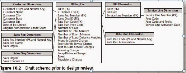
Customer Dimension

The conformed customer dimension is a critical element for effective CRM. A

well-maintained, well-deployed conforming customer dimension is the cornerstone

of sound customer-centric analysis.

The customer dimension is typically the most challenging dimension for any

data warehouse. In a large organization, the customer dimension can be

extremely deep (with millions of rows), extremely wide (with dozens or even

hundreds of attributes), and sometimes subject to rather rapid change. One

leading direct marketer maintains over 3,000 attributes about its customers.

Any organization that deals with the general public needs an individual

human being dimension. The biggest retailers, credit card companies, and

government agencies have monster customer dimensions whose sizes exceed

100 million rows. To further complicate matters, the customer dimension often

represents an amalgamation of data from multiple internal and external source

systems.

Dimension Outrigger

Dimension Outriggers for a Low-Cardinality Attribute Set

As we said in Chapter 2, a dimension is said to be snowflaked when the low-cardinality

columns in the dimension have been removed to separate normalized

tables that then link back into the original dimension table. Generally,

snowflaking is not recommended in a data warehouse environment because it

almost always makes the user presentation more complex, in addition to having

a negative impact on browsing performance. Despite this prohibition

against snowflaking, there are some situations where you should build a

dimension outrigger that has the appearance of a snowflaked table. Outriggers

have special characteristics that cause them to be permissible snowflakes.

In Figure 6.3, the dimension outrigger is a set of data from an external data

provider consisting of 150 demographic and socioeconomic attributes regarding

the customers’ county of residence. The data for all customers residing in a given

county is identical. Rather than repeating this large block of data for every customer

within a county, we opt to model it as an outrigger. There are several factors

that cause us to bend our no-snowflake rule. First of all, the demographic

data is available at a significantly different grain than the primary dimension

data (county versus individual customer). The data is administered and loaded

at different times than the rest of the data in the customer dimension. Also, we

really do save significant space in this case if the underlying customer dimension

is large. If you have a query tool that insists on a classic star schema with no

snowflakes, you can hide the outrigger under a view declaration.

Dimension outriggers are permissible, but they should be the exception rather than

the rule. A red warning flag should go up if your design is riddled with outriggers;

you may have succumbed to the temptation to overly normalize the design.

Large Changing Customer Dimensions

Multimillion-row customer dimensions present two unique challenges that

warrant special treatment. Even if a clean, flat dimension table has been implemented,

it generally takes too long to constrain or browse among the relationships

in such a big table. In addition, it is difficult to use our tried-and-true

techniques from Chapter 4 for tracking changes in these large dimensions. We

probably don’t want to use the type 2 slowly changing dimension technique

and add more rows to a customer dimension that already has millions of rows

in it. Unfortunately, huge customer dimensions are even more likely to change

than moderately sized dimensions. We sometimes call this situation a rapidly

changing monster dimension!

minidimension

Business users often want to track the myriad of customer attribute changes.

In some businesses, tracking change is not merely a nice-to-have analytic capability.

Insurance companies, for example, must update information about their

customers and their specific insured automobiles or homes because it is critical

to have an accurate picture of these dimensions when a policy is approved

or claim is made.

Fortunately, a single technique comes to the rescue to address both the browsing-

performance and change-tracking challenges. The solution is to break off

frequently analyzed or frequently changing attributes into a separate dimension,

referred to as a minidimension. For example, we could create a separate

minidimension for a package of demographic attributes, such as age, gender,

number of children, and income level, presuming that these columns get used

extensively. There would be one row in this minidimension for each unique

combination of age, gender, number of children, and income level encountered

in the data, not one row per customer. These columns are the ones that

are analyzed to select an interesting subset of the customer base. In addition,

users want to track changes to these attributes. We leave behind more constant

or less frequently queried attributes in the original huge customer table.

Sample rows for a demographic minidimension are illustrated in Table 6.3.

When creating the minidimension, continuously variable attributes, such as

income and total purchases, should be converted to banded ranges. In other

words, we force the attributes in the minidimension to take on a relatively small

number of discrete values. Although this restricts use to a set of predefined

bands, it drastically reduces the number of combinations in the minidimension.

If we stored income at a specific dollar and cents value in the minidimension,

when combined with the other demographic attributes, we could end up with as

many rows in the minidimension as in the main customer dimension itself. The

use of band ranges is probably the most significant compromise associated

with the minidimension technique because once we decide on the value bands,

it is quite impractical to change to a different set of bands at a later time. If users

insist on access to a specific raw data value, such as a credit bureau score that is

updated monthly, it also should be included in the fact table, in addition to

being represented as a value band in the demographic minidimension.

Values are available in mididimension as well as in fact

Every time we build a fact table row, we include two foreign keys related to the

customer: the regular customer dimension key and the minidimension demographics

key. As shown in Figure 6.4, the demographics key should be part of

the fact table’s set of foreign keys in order to provide efficient access to the fact

table through the demographics attributes. This design delivers browsing and

constraining performance benefits by providing a smaller point of entry to the

facts. Queries can avoid the huge customer dimension table altogether unless

attributes from that table are constrained.

When the demographics key participates as a foreign key in the fact table,

another benefit is that the fact table serves to capture the demographic profile

changes. Let’s presume that we are loading data into a periodic snapshot fact

table on a monthly basis. Referring back to our sample demographic minidimension

sample rows in Table 6.3, if one of our customers, John Smith, was 24

years old with an income of $24,000, we’d begin by assigning demographics

key 2 when loading the fact table. If John has a birthday several weeks later,

we’d assign demographics key 18 when the fact table was next loaded. The

demographics key on the earlier fact table rows for John would not be

changed. In this manner, the fact table tracks the age change. We’d continue to

assign demographics key 18 when the fact table is loaded until there’s another

change in John’s demographic profile. If John receives a raise to $26,000 several

months later, a new demographics key would be reflected in the next fact

table load. Again, the earlier rows would be unchanged. Historical demographic

profiles for each customer can be constructed at any time by referring

to the fact table and picking up the simultaneous customer key and its contemporary

demographics key, which in general will be different from the most

recent demographics key.

The minidimension terminology refers to when the demographics key is part of the

fact table composite key; if the demographics key is a foreign key in the customer dimension,

we refer to it as an outrigger.

The best approach for efficiently browsing and tracking changes of key attributes in

really huge dimensions is to break off one or more minidimensions from the dimension

table, each consisting of small clumps of attributes that have been administered

to have a limited number of values.

Variable-Width Attribute Set

When using external prospect lists, we often are permitted only a one-time use

of the list and don’t have the legal right to store the prospect information internally.

However, if we’ve generated our own prospect information, it certainly

can be stored in the data warehouse. Let’s assume that we’re capturing metrics,

perhaps associated with solicitation or quote-generation events that apply to

both prospects and customers. We could store the prospects and customers

together in a single contact dimension; however, there is a significant disparity

between the numbers of attributes for prospective versus customer contacts. As

illustrated in Figure 6.6, we may know only a handful of identification and location

attributes about our prospects. On the other hand, we may know 50 additional

attributes for a customer, covering purchase, payment, credit and service

behaviors, directly elicited profile attributes, and third-party purchased demographic

attributes. In the world of electronic retailing, we can equate prospects

to be the anonymous Web site visitors as opposed to our registered customers

If we’re dealing with a database platform that supports variable-width rows,

such as Oracle, we may be able to build a single dimension with the full complement

of attributes if the total attributes list is not too long; in some of these

cases, we don’t need to worry about all the prospects’ null columns because

they take up virtually zero disk space. However, if we have a fixed-width database,

or if the attributes list is very long, we are uncomfortable with all the

empty columns for the prospects. In this case, as shown in Figure 6.6, we break

the dimension into a 10-million-row base dimension table consisting of attributes

that are common to both prospects and customers, along with a 1-millionrow

customer minidimension that contains the additional attributes we know

about our customers. Again, we include two foreign keys in the fact table.

Nine of ten fact table rows would join to an empty customer row in the

extended customer minidimension.

behaviour customer group

The secret to building complex behavioral study group queries is to capture the keys

of the customers or products whose behavior you are tracking. You then use the captured

keys to constrain other fact tables without having to rerun the original behavior

analysis.

Variable-Depth Hierarchies

Representing an arbitrary, ragged organization hierarchy is an inherently difficult

task in a relational environment. For example, we may want to report the

revenues for a set of commercial customers who have intricate relationships

with each other, such as in Figure 6.8. Each square on the diagram represents

an individual customer entity connected in an organizational tree. The illustrated

organization has four levels; other customer organizations may have

one, ten, or more levels. Let’s assume that we sell our products or services to

any of these commercial customers. Thus the customer dimension rows can

play the role of parent as well as child. We may want to look at the customers

and their sales revenue individually. At other times, we may want to summarize

revenue to any node in the overall organizational tree.

Instead of using a recursive pointer, we insert a bridge table between the customer

dimension and fact tables, as depicted in Figure 6.9. The bridge table has

been called a helper or associative table in the past, but going forward, we’ll consistently

use the bridge terminology. Use of the bridge table is optional; neither

the customer dimension table nor the fact table has to be modified in any way.

If the bridge table is left out, the customer dimension table joins to the fact

table in the usual way. We can report revenue by customer, but we’re unable to

navigate the organization hierarchy. When the bridge table is inserted between

the customer dimension and fact tables, we’re able to analyze revenue results

at any hierarchical level using standard SQL, albeit via a more complicated

presentation.

The bridge table contains one row for each pathway in Figure 6.8 from a customer

entity to each subsidiary beneath it, as well as a row for the zero-length pathway

from a customer to itself. Each pathway row contains the customer key of the parent

roll-up entity, the customer key of the subsidiary entity, the number of levels

between the parent and the subsidiary, a bottom-most flag that identifies a subsidiary

with no further nodes beneath it, and finally, a top-most flag to indicate

that there are no further nodes above the parent. The sample bridge table rows

corresponding to the hierarchy in Figure 6.8 are shown as in Table 6.4.

When we want to descend the organization hierarchy, we join the tables

together as shown in Figure 6.9. We can now constrain the customer table to a

particular parent customer and request any aggregate measure of all the subsidiaries

at or below that customer. We can use the “# of Levels from Parent”

column in the organization bridge table to control the depth of the analysis.

Constraining to a value of 1 would give all the direct subsidiaries of the customer.

A value greater than zero would give all subsidiary customers but not

the original parent. We can use the “Bottom Flag” column to jump directly to all

the bottom-most customer entities but omit all higher-level customer entities.

If we wanted

to sum up revenue in the fact table for a given customer and all its subsidiaries,

the SQL code would look something like the following:

We can request all the revenue from the organizations associated with many

parents at once, but we have to get the subsidiary keys distinctly or risk double

counting. In the following example we retrieve the January 2002 revenue

from all organizations whose parents are located in San Francisco. The SQL

code is messier, but it works for both unique and multiple parent customers.

Be very careful when simultaneously joining a single dimension table to two fact

tables of different cardinality. In many cases, relational systems will return the

wrong answer. A similar problem arises when joining two fact tables of different

granularity together directly.

Consider the case in which we have a fact table of customer solicitations and

another fact table with the customer responses resulting both from the solicitations

and other independent sources. There is a one-to-many relationship

between customer and solicitation and another one-to-many relationship

between customer and response. The solicitation and response fact tables have

different cardinalities; in other words, not every solicitation results in a

response (unfortunately for the marketing department), and some responses

are received for which there is no solicitation. Simultaneously joining the solicitation

fact table to the customer dimension, which is in turn joined to the

response fact table, does not return the correct answer in a relational DBMS

because of the cardinality differences. Fortunately, this problem is easily

avoided. We simply issue multipass SQL code to query the solicitation and

response tables in separate queries and then outer join the two answer sets.

The multipass approach has additional benefits in terms of better controlling

performance parameters, in addition to supporting queries that combine data

from fact tables in different physical locations.

Chapter 7 : Accounting

General Ledger Data
The general ledger (G/L) is a core foundation financial system because it ties
together the detailed information collected by the purchasing, payables (what
you owe to others), and receivables (what others owe you) subledgers or systems.
In this case study we’ll focus on the general ledger rather than the subledgers,
which would be handled as separate business processes and fact tables.
As we work through a basic design for G/L data, we discover, once again, that
two complementary schemas with periodic snapshot and transaction-grained
fact tables working together are required.
Financial analysts are constantly looking to streamline the processes for
period-end closing, reconciliation, and reporting of G/L results. While operational
G/L systems often support these requisite capabilities, they may be
cumbersome, especially if you’re not dealing with a modern G/L. In this chapter
we’ll focus on more easily analyzing the closed financial results rather than
facilitating the close. However, in many organizations, G/L trial balances are
loaded into the data warehouse to leverage the capabilities of the data warehouse’s
presentation area to find the needles in the G/L haystack and then
make the appropriate operational adjustments before the period ends.
The sample schema in Figure 7.1 supports the access and analysis of G/L
account balances at the end of each account period. It would be very useful for
many kinds of financial analysis, such as account rankings, trending patterns,

and period-to-period comparisons.

In general, to-date totals should be calculated, not stored in the fact table.

Role of OLAP and Packaged Analytic Solutions

Given the standard nature of G/L processing, purchasing a G/L package

rather than attempting to build one from scratch has been a popular route for

years. Nearly all the operational package providers also offer a complementary

analytic solution, sometimes in partnership with one of the multidimensional

OLAP vendors. In many cases these canned analyses based on the

cumulative experience of the vendor are a sound way to jump-start a financial

data warehouse implementation with potentially reduced cost and risk. The

analytic solutions often have tools to assist with the extraction and staging of

operational financial data, as well as tools to assist with analysis and interpretation.

However, as we discussed in Chapter 6, when leveraging packaged

solutions, we need to be cautious about avoiding stovepipe applications. One

could easily find oneself in a situation with separate financial, CRM, human

resources, and ERP packaged analytic solutions from as many different vendors,

none of which integrates with other internal data. We need to conform

dimensions across the entire data warehouse environment regardless of

whether we’re building our own solution or implementing packages. Packaged

analytic solutions can turbocharge your data warehouse implementation;

however, they do not alleviate the need for conformance. Most

organizations inevitably will rely on a combination of building, buying, and

integrating for a complete solution

The budget line item identifies the purpose of the proposed spending, such as

employee wages or office supplies. Typically, several levels of summarization

categories are associated with a budget line item. As we discussed in Chapter 5,

all the budget line items may not have the same number of levels in their summarization

hierarchy, such as when some have only a category roll-up but not

a subcategory. In this case we may populate the dimension attributes by replicating

the category name in the subcategory column to avoid having line items

roll up to a “Not Applicable” subcategory bucket. The budget line-item dimension

also would identify the budget year and budget version.

The effective month is the month during which the budget changes are posted.

The first entries for a given budget year would show the effective month when

the budget is first approved. If the budget is updated or modified as the budget

year gets underway, the effective months would occur during the budget

year. If we don’t adjust the budget at all throughout the year, then the only

entries would be the first ones when the budget is approved. This is what we

meant when we specified the grain to be the net change. It is critical that you

understand this point, or you won’t understand what is in this budget fact

table or how it is used.

Consolidated Fact Tables

When facts from multiple business processes are combined in a consolidated fact

table, they must live at the same level of granularity and dimensionality. Optimally, the

separate facts naturally live at a common grain. Otherwise, we are forced to eliminate

or aggregate some dimensions to support the one-to-one correspondence or keep

them in separate fact tables. Project teams should not create artificial facts or dimensions

in an attempt to force fit the consolidation of differently grained fact data

Chapter 8 : Human Resource Management

Time-Stamped Transaction Tracking in a Dimension
Thus far the dimensional models we have designed closely resemble each other
in that the fact tables have contained key performance metrics that typically can
be added across all the dimensions. It is easy for dimensional modelers to get
lulled into a kind of additive complacency. In most cases, this is exactly how it is
supposed to work. However, with HR employee data, many of the facts aren’t
additive. Most of the facts aren’t even numbers, yet they are changing all the time.


Factless Fact Table

We envision using the type 2 slowly changing dimension technique for tracking

changed profile attributes in the employee dimension. Consequently,

with every employee transaction in the fact table in Figure 8.1, we also create

a new type 2 row in the employee dimension that represents the employee’s

profile as a result of the transaction event. It continues to accurately describe

the employee until the next employee transaction occurs at some indeterminate

time in the future. The alert reader is quick to point out that we’ve

designed an employee transaction fact table and a type 2 employee dimension

table with the exact same number of rows, which are almost always

joined to one another. At this point dimensional modeling alarms should be

going off. We certainly don’t want to have as many rows in a fact table as we

do in a related dimension table.

Time-Stamped Dimension with Periodic Snapshot Facts

In addition to profiling the employee base in HR, we also need to report summary

statuses of the employee base on a regular, monthly basis. We’re interested

in counts, statistics, and totals, including such things as number of

employees, total salary paid during the month, vacation days taken, vacation

days accrued, number of new hires, and number of promotions. We want to

analyze the data by all possible slices, including time and organization. We

need to access totals at the end of each month, even when there is no transaction

activity in a given employee’s profile during that month.

As shown in Figure 8.3, the HR periodic snapshot consists of a fairly ordinary

looking fact table with three dimensions: month, employee transaction, and

organization. The month dimension table contains the usual descriptors for

the corporate calendar at the month grain. The employee transaction key in a

fact table row is the employee transaction key that was effective on the last day

of the given reporting month. This guarantees that the month-end report is a

correct depiction of all the employee profiles. The organization dimension

contains a description of the organization to which the employee belongs at

the close of the relevant month.

Audit Dimension

Keyword Outrigger Dimension

The skills group identifies a given set of skills keywords. All IT employees

who are proficient in Oracle, Unix, and SQL would be assigned the same skills

group key. In the skills group outrigger, there would be three rows for this particular

group, one for each of the associated keyword skills (Oracle, Unix, and

SQL). In this case, just two attributes are associated with each skill, description

and category, so we include these attributes in the outrigger directly.

Survey Questionnaire Data

In order to analyze questionnaire data, we create a fact table with one row for

each question on a respondent’s survey, as illustrated in Figure 8.7. There

would be two role-playing employee dimensions in the schema corresponding

to the responding employee and the reviewed employee. The survey dimension

consists of descriptors about the survey instrument. The question dimension

would provide the question and its categorization. Presumably, the same

question is asked on multiple surveys. The survey and question dimensions

can be useful handles for searching for specific topics in a broad database of

questionnaires. The response dimension contains the responses and perhaps

categories of responses, such as favorable or hostile

Chapter 9 : Financial Services

The financial services industry encompasses a wide variety of businesses,

including credit card companies, brokerage firms, and mortgage providers.

This chapter will focus primarily on retail banks given that most readers have

some degree of personal familiarity with this type of financial institution. A

full-service bank offers a breadth of products, including checking accounts,

savings accounts, mortgage loans, personal loans, credit cards, and safe

deposit boxes. This chapter begins with a very simplistic schema. We then

explore several schema extensions, including handling of the bank’s broad

portfolio of heterogeneous products that vary significantly by line of business

Causal dimensions. These dimensions, such as promotion, contract, deal,

store condition, or even weather, provide additional insight into the cause

of an event.

Multiple date or time-stamp dimensions. Refer to Chapter 5 for sample fact

tables with multiple date stamps, especially when the fact table is an accumulating

snapshot.

Degenerate dimensions. These dimensions identify operational transaction

control numbers, such as an order, invoice, bill of lading, or ticket, as illustrated

initially in Chapter 2.

Role-playing dimensions. Role-playing occurs when a single physical

dimension appears several times in a fact table, each represented as a

separate logical table with unique column names through views.

Status dimensions. These dimensions identify the current status of a transaction

or monthly snapshot within some larger context, such as an account

status.

Audit dimension. As discussed in Chapter 8, this dimension is designed to

track data lineage and quality.

Junk dimensions. These consist of correlated indicators and flags, as

described in Chapter 5.

Minidimensions

It is unreasonable to rely on the type 2 SCD technique to track changes in the

account dimension given the dimension row count and attribute volatility,

such as the monthly update of credit bureau attributes. Instead, we break off

the browseable and changeable attributes into multiple minidimensions, such

as credit bureau and demographics minidimensions, whose keys are included

in the fact table. This recommendation was illustrated in Figure 6.4. The minidimensions

allow us to slice and dice the fact data based on a lengthy list of

attributes while readily tracking attribute changes over time, even though they

may be updated at different frequencies. While minidimensions are extremely

powerful, we need to be careful that we don’t overuse the technique. However,

account-oriented financial services are a good environment for using the minidimension

technique because the primary fact table is a very long-running

periodic snapshot. Thus a fact table row exists for every account every month.

This fact row provides a home for all the foreign keys and links them together

so that we can always see the account together with all the other minidimensions

for any month.

Minidimensions should consist of correlated clumps of attributes; each attribute

shouldn’t be its own minidimension or we’d end up with too many dimensions

in the fact table.

As described in Chapter 6, one of the compromises associated with minidimensions

is the need to band attribute values in order to maintain reasonable

minidimension row counts. Rather than storing extremely discrete income

amounts, such as $31,257.98, we store income ranges, such as $30,000-$34,999

in the minidimension. Similarly, the profitability scores may range from 1

through 1,200, which we band into fixed ranges such as less than or equal to

100, 101-150, 151-200, and so on in the minidimension.

Household Dimension

From the bank’s perspective, a household may be comprised of several

accounts and individual account holders. For example, consider John and

Mary Smith as a single household. John has a checking account, and Mary has

a savings account. In addition, John and Mary have a joint checking account,

credit card, and mortgage with the bank. All five of these accounts are considered

to be a part of the same Smith household despite the fact that minor

inconsistencies may exist in the operational name and address information

The decision to treat accounts and households as separate dimensions is somewhat

a matter of the designer’s prerogative. Despite the fact that accounts and

households are correlated intuitively, we decide to treat them separately

because of the size of the account dimension and the volatility of the account

constituents within a household dimension, as referenced earlier.

Multivalued Dimensions

As we just saw in the John and Mary Smith example, an account can have one,

two, or more individual account holders, or customers, associated with it.

Obviously, we cannot merely include the customer as an account attribute;

doing so violates the granularity of the dimension table because more than one

individual can be associated with an account. Likewise, we cannot include

customer as an additional dimension in the fact table; doing so violates the

granularity of the fact table (one row per account per month) again because

more than one individual can be associated with any given account. This is a

classic example of a multivalued dimension, which we’ll develop fully in

Chapter 13. For now, suffice it to say that to link an individual customer

dimension to an account-grained fact table requires the use of an account-tocustomer

bridge table, as shown in Figure 9.3. At a minimum, the primary key

of the bridge table consists of the surrogate account and customer foreign

keys.

An open-ended many-valued attribute can be associated with a dimension row by

using a bridge table to associate the many-valued attributes with the dimension

Point-in-Time Balances

Assuming that business requirements already have driven the need to make

transaction detail data available for analysis, we could leverage this transaction

detail to determine an arbitrary point-in-time balance. To simplify matters,

we’ll boil the account transaction fact table down to an extremely simple

design, as illustrated in Figure 9.5. The transaction type key joins to a small

dimension table of permissible transaction types. The transaction sequence

number is a continuously increasing numeric number running for the

lifetime of the account. The final flag indicates whether this is the last

transaction for an account on a given day. The transaction amount is selfexplanatory.

The balance fact is the ending account balance following the

transaction event.

Like all transaction-grained fact tables, we add a row to the fact table in

Figure 9.5 only if a transaction occurs. If an account were quiet for two weeks,

perhaps January 1 through 14, there would be no rows in the fact table for the

account during that time span.

Leveraging the transaction fact table for dual purposes requires that the fact

table is absolutely complete and accurate. Every transaction against the

account must appear in this fact table, or else the running balance will not be

accurate. A late-arriving transaction row would require sweeping forward

from the point of insertion in that account and incrementing all the balances

and transaction sequence numbers. Note that we haven’t explicitly used the

transaction sequence number in this discussion, although it is needed in this

design to reconstruct the true sequence of transactions reliably and to provide

the basis of the fact table’s primary key, which is the date, account, and

sequence number. We prefer using the sequence number rather than a time-ofday

stamp because differences between the sequence numbers are a valid measure

of account activity.

Heterogeneous Product Schemas

The keys of the custom product dimensions are the same keys used in the core

product dimension, which contains all possible product keys. For example, if

the bank offers a $500 minimum balance with no per-check charge checking

product, the product would have the same surrogate key in both the core and

custom checking product dimensions. As we discussed in Chapter 3, establishing

conformed dimensions is essential to an extensible data warehouse

architecture. Each custom product dimension is a subset of rows from the core

product dimension table. Each custom product dimension contains attributes

specific to a particular product type.

This heterogeneous product technique obviously applies to any business that

offers widely varied products through multiple lines of business. If we worked

for a technology company that sells hardware, software, and services, we can

imagine building core sales fact and product dimension tables to deliver the

global customer perspective. The core tables would include all facts and

dimension attributes that are common across lines of business. The core tables

would then be supplemented with schemas that do a deep dive into custom

facts and attributes that vary by business. Again, a specific product would be

assigned the same surrogate product key in both the core and custom product

dimensions.

A family of core and custom fact tables is needed when a business has heterogeneous

products that have naturally different facts and descriptors but a single

customer base that demands an integrated view

Context-dependent dimension outriggers

In the case of account-oriented financial services, when a product is sold to a

customer, a new account is opened. In the case of some banking products, such

as mortgages, more account-specific descriptive information is collected when

the account opening occurs. For example, the bank may offer a 15-year fixedrate

mortgage at a given rate. When the mortgage originates, the bank will

know more about the specific property, including the address, appraised

value, square footage, home type (for example, single-family, townhouse, condominium,

trailer), construction type (for example, wood frame, brick,

stucco), date of construction, and acreage. These attribute values differ by

account, so they don’t belong in the what-the-bank-sells product dimension.

As shown in Figure 9.7, we can envision an account dimension outrigger for

some account types

Chapter 10 : Telecommunication

Geographic Location Dimension

Let’s shift gears and presume that we’re now working for a phone company

with land lines tied to a specific physical location. In general, the telecommunications

industry has a very well-developed notion of location. The same

could be said for the utilities industry. Many of its dimensions contain a precise

geographic location as part of the attribute set. The location may be resolved to

a physical street, city, state, and ZIP code or even to a specific latitude and longitude.

Using our dimension role-playing technique, we imagine building a

single master location table where data is standardized once and then reused.

The location table could be part of the service line telephone number, equipment

inventory, network inventory (including poles and switch boxes), real

estate inventory, service location, dispatch location, right of way, and even customer

entities. Each row in the master location table is a specific point in space

that rolls up to every conceivable geographic grouping, such as census tracts

and counties. A location could roll up to multiple unique geographic groupings

simultaneously.

Chapter 11 : Transportation

Multiple Fact Table Granularity

When it comes to the grain, we encounter a situation in this case where we are

presented with multiple potential levels of fact table granularity. Each of these

levels of granularity has different metrics associated with them.

At the most granular level, the airline captures data at the leg level. The leg

represents an aircraft taking off at one airport and landing at another without

any intermediate stops. Capacity planning and flight scheduling analysts are

very interested in this discrete level of information because they’re able to look

at the number of seats to calculate load factors by leg. We also can include facts

regarding the leg’s flight duration as well as the number of minutes late at

departure and arrival. Perhaps there’s even a dimension to easily identify

on-time arrivals.

The next level of granularity corresponds to a segment. In this case we’re

looking at the portion of a trip on a single aircraft. Segments may have one or

more legs associated with them. If you take a flight from San Francisco to

Minneapolis with a stop in Denver but no aircraft change, you have flown one

segment (SFO-MSP) but two legs (SFO-DEN and DEN-MSP). Conversely, if

the flight flew nonstop from San Francisco to Minneapolis, you would have

flown one segment as well as one leg. The segment represents the line item on

an airline ticket coupon; revenue and mileage credit is generated at the segment

level.

Next, we can analyze flight activity by trip. The trip provides an accurate picture

of customer demand. In our prior example, assume that the flights from

San Francisco to Minneapolis required the flyer to change aircraft in Denver. In

this case the trip from San Francisco to Minneapolis would entail two segments

corresponding to the two aircraft involved. In reality, the passenger just

asked to go from San Francisco to Minneapolis; the fact that he or she needed

to stop in Denver was merely a necessary evil but certainly wasn’t requested.

For this reason, sales and marketing analysts are interested in trip-level data.

Linking Segments into Trips

Despite the powerful dimensional framework we just designed, we are unable

to easily answer one of the most important questions about our frequent flyers,

namely, where are they going? The segment grain masks the true nature of

the trip. If we fetch all the segments of the airline voyage and sequence them

by segment number, it is still nearly impossible to discern the trip start and end

points. Most complete itineraries start and end at the same airport. If a lengthy

stop were used as a criterion for a meaningful trip destination, it would

require extensive and tricky processing whenever we tried to summarize a

number of voyages by the meaningful stops.

The answer is to introduce two more airport role-playing dimensions: trip origin

and trip destination, while keeping the grain at the flight segment level.

These are determined during data extraction by looking on the ticket for any

stop of more than four hours, which is the airline’s official definition of a

stopover. The enhanced schema looks like Figure 11.2. We would need to exercise

some caution when summarizing data by trip in this schema. Some of the

dimensions, such as fare basis or class of service flown, don’t apply at the trip

level. On the other hand, it may be useful to see how many trips from San

Francisco to Minneapolis included an unrestricted fare on a segment

In addition to linking segments into trips as Figure 11.2 illustrates, if the business

users are constantly looking at information at the trip level, rather than by segment,

we might be tempted to create an aggregate fact table at the trip grain.

Some of the earlier dimensions discussed, such as class of service, fare basis, and

flight, obviously would not be applicable. The facts would include such metrics

as trip gross revenue and additional facts that would appear only in this complementary

trip summary table, such as the number of segments in the trip.

However, we would only go to the trouble of creating such an aggregate table if

there were obvious performance or usability issues when we used the segmentlevel

table as the basis for rolling up the same reports. If a typical trip consisted

of three segments, then we might barely see a three times performance improvement

with such an aggregate table, meaning that it may not be worth the bother.

Cargo Shipper

The schema for a cargo shipper looks quite similar to the frequent flyer schemas

just developed. Suppose that a transoceanic shipping company transports bulk

goods in containers from foreign to domestic ports. The items in the containers

are shipped from an original shipper to a final consignor. The trip can have multiple

stops at intermediate ports. It is possible that the containers may be offloaded

from one ship to another at a port. Likewise, it is possible that one or

more of the legs may be by truck rather than ship.

As illustrated in Figure 11.3, the grain of the fact table is the container on a specific

bill-of-lading number on a particular leg of its trip.

The ship mode dimension identifies the type of shipping company and specific

vessel. The item dimension contains a description of the items in a container.

The container dimension describes the size of the container and whether it

requires electrical power or refrigeration. The commodity dimension describes

one type of item in the container. Almost anything that can be shipped can be

described by harmonized commodity codes, which are a kind of master conformed

dimension used by agencies, including U.S. Customs. The consignor

foreign transporter, foreign consolidator, shipper, domestic consolidator,

domestic transporter, and consignee are all roles played by a master business

entity dimension that contains all the possible business parties associated with

a voyage. The bill-of-lading number is a degenerate dimension. We assume that

the fees and tariffs are applicable to the individual leg of the voyage.

Travel Services

If we work for a travel services company, we can envision complementing the

customer flight activity schema with fact tables to track associated hotel stays

and rental car usage. These schemas would share several common dimensions,

such as the date, customer, and itinerary number, along with ticket and

segment number, as applicable, to allow hotel stays and car rentals to be interleaved

correctly into a airline trip. For hotel stays, the grain of the fact table is

the entire stay, as illustrated in Figure 11.4. The grain of a similar car rental fact

table would be the entire rental episode. Of course, if we were constructing a

fact table for a hotel chain rather than a travel services company, the schema

would be much more robust because we’d know far more about the hotel property

characteristics, the guest’s use of services, and associated detailed charges

Combining Small Dimensions into a Superdimension

We stated previously that if a many-to-many relationship exists between two

groups of dimension attributes, then they should be modeled as separate

dimensions with separate foreign keys in the fact table. Sometimes, however,

we’ll encounter a situation where these dimensions can be combined into a

single superdimension rather than treating them as two separate dimensions

with two separate foreign keys in the fact table

Class of Service

The Figure 11.1 draft schema included the class of service flown dimension. Following

our first design checkpoint with the business community, we learn that

the business users want to analyze the class of service purchased, as well as the

class flown. Unfortunately, we’re unable to reliably determine the class of service

actually used from the original fare basis because the customer may do a

last-minute upgrade. In addition, the business users want to easily filter and

report on activity based on whether an upgrade or downgrade occurred. Our

initial reaction is to include a second role-playing dimension and foreign key in

the fact table to support access to both the purchased and flown class of service,

along with a third foreign key for the upgrade indicator. In this situation, however,

there are only three rows in each class dimension table to indicate first,

business, and coach classes. Likewise, the upgrade indicator dimension also

would have just three rows in it, corresponding to upgrade, downgrade, or no

class change. Since the row counts are so small, we elect instead to combine the

dimensions into a single class of service dimension, as illustrated in Figure 11.5.

In most cases, role-playing dimensions should be treated as separate logical dimensions

created via views on a single physical table, as we’ve seen earlier with date

dimensions. In isolated situations it may make sense to combine the separate

dimensions into a superdimension, notably when the data volumes are extremely

small or there is a need for additional attributes that depend on the combined

underlying roles for context and meaning.

Country-specific calendar outrigger.

If there’s no need to roll up or filter on time-of-day groups, then we have the

option to treat time as a simple numeric fact instead. In this situation, the time

of day would be expressed as a number of minutes or number of seconds since

midnight, as shown in Figure 11.8

Date and Time in Multiple Time Zones

When operating in multiple countries or even just multiple time zones, we’re

faced with a quandary concerning transaction dates and times. Do we capture

the date and time relative to local midnight in each time zone, or do we express

the time period relative to a standard, such as the corporate headquarters

date/time or Greenwich Mean Time (GMT)? To fully satisfy users’ requirements,

the correct answer is probably both. The standard time allows us to see

the simultaneous nature of transactions across the business, whereas the local

time allows us to understand transaction timing relative to the time of day.

Contrary to popular belief, there are more than 24 time zones (corresponding

to the 24 hours of the day) in the world. For example, there is a single time

zone in India, offset from GMT by 5.5 or 6.5 hours depending on the time of

year. The situation gets even more unpleasant when you consider the complexities

of switching to and from daylight saving time. As such, it’s unreasonable

to think that merely providing an offset in a fact table can support

equivalized dates and times. Likewise, the offset can’t reside in a time or airport

dimension table. The recommended approach for expressing dates and

times in multiple time zones is to include separate date and time-of-day

dimensions (or time-of-day facts, as we just discussed) corresponding to the

local and equivalized dates, as shown in Figure 11.9.

Chapter 12 : Education

In the case of applicant tracking, prospective students progress through a

standard set of admissions hurdles or milestones. Perhaps we’re interested in

tracking activities around key dates, such as receipt of preliminary admissions

test scores, information requested (via Web or otherwise), information sent,

interview conducted, on-site campus visit, application received, transcript

received, test scores received, recommendations received, first pass review by

admissions, review for financial aid, final decision from admissions, accepted,

244 CHAPT E R 12

admitted, and enrolled. At any point in time, people in the admissions and

enrollment management area are interested in how many applicants are at

each stage in the pipeline. The process is much like a funnel, where many

applicants enter the pipeline, but far fewer progress through to the final stage.

Admission personnel also would like to analyze the applicant pool by a variety

of characteristics.

The grain of the accumulating snapshot to track the applicant’s lifecycle is one

row per prospective student. This granularity represents the lowest level of

detail captured when the prospect enters the pipeline. As more information is

collected while the prospect progresses toward application, acceptance, and

admission, we continue to revisit and update the prospect’s status in the fact

table row, as illustrated in Figure 12.1.

Student Registration Events

There are many situations in which events need to be recorded as the simultaneous

coming together of a number of dimensional entities. For example, we

can track student registrations by term. The grain of the fact table would be

one row for each registered course by student and term. As illustrated in Figure

12.2, the fact table has the following dimensionality: term, student, student

major and attainment, course, and faculty.

In this scenario we’re dealing with fact data at the term level rather than at the

more typical calendar day, week, or month granularity. Term is the lowest level

available for the registration events. The term dimension still should conform

to the calendar date dimension. In other words, each date in our daily calendar

dimension should identify the term (for example, Fall AY2002), academic year

(for example, AY2002), and term season (for example, Winter). The column

labels and values must be identical for the attributes common to both the

calendar date and term dimensions

Events often are modeled as a fact table containing a series of keys, each representing

a participating dimension in the event. Event tables often have no obvious numeric

facts associated with them and hence are called factless fact tables.

The inevitable confusion surrounding the SQL statement, while not a serious

semantic problem, causes some designers to create an artificial implied fact,

perhaps called registration count (as opposed to dummy), that is always populated

by the value 1. While this fact does not add any information to the fact

table, it makes the SQL more readable, such as:

SELECT FACULTY, SUM(REGISTRATION_COUNT)... GROUP BY FACULTY

At this point the table is no longer strictly factless, but most would agree that

the 1 is nothing more than an artifact.

Explicit Rows for What Didn’t Happen

Perhaps people are interested in monitoring students who were registered for

a course but didn’t show up. In this example we can envision adding explicit

rows to the fact table for attendance events that didn’t occur. Adding rows is

viable in this scenario because the nonattendance events have the same exact

dimensionality as the attendance events. Likewise, the fact table won’t grow at

an alarming rate, presuming (or perhaps hoping) that the no shows are a small

percentage of the total students registered for a course. In this situation we’re

no longer dealing with a factless fact table because now the attendance fact

would equal either 1 or 0.

While this approach is reasonable in this scenario, creating rows for events that

didn’t happen is ridiculous in many situations. For example, if we think back

to our transportation case study, we certainly don’t want to build fact table

rows for each flight not taken by a frequent flyer on a given day.